Database Management Systems (DBMS)

 What is Database

The database is a collection of inter-related data which is used to retrieve, insert and delete the data efficiently. It is also used to organize the data in the form of a table, schema, views, and reports, etc.

For example: The college Database organizes the data about the admin, staff, students and faculty etc.

Using the database, you can easily retrieve, insert, and delete the information.

Database Management System

o    Database management system is a software which is used to manage the database. For example: MySQL, Oracle, etc are a very popular commercial database which is used in different applications.

Characteristics of DBMS

o    It uses a digital repository established on a server to store and manage the information.

o    It can provide a clear and logical view of the process that manipulates data.

o    DBMS contains automatic backup and recovery procedures.

o    It contains ACID properties which maintain data in a healthy state in case of failure.

o    It can reduce the complex relationship between data.

o    It is used to support manipulation and processing of data.

o    It is used to provide security of data.

o    It can view the database from different viewpoints according to the requirements of the user.

 

Advantages of DBMS

o    Controls database redundancy: It can control data redundancy because it stores all the data in one single database file and that recorded data is placed in the database.

o    Data sharing: In DBMS, the authorized users of an organization can share the data among multiple users.

o    Easily Maintenance: It can be easily maintainable due to the centralized nature of the database system.

o    Reduce time: It reduces development time and maintenance need.

o    Backup: It provides backup and recovery subsystems which create automatic backup of data from hardware and software failures and restores the data if required.

o    multiple user interface: It provides different types of user interfaces like graphical user interfaces, application program interfaces

Disadvantages of DBMS

o    Cost of Hardware and Software: It requires a high speed of data processor and large memory size to run DBMS software.

o    Size: It occupies a large space of disks and large memory to run them efficiently.

o    Complexity: Database system creates additional complexity and requirements.

o    Higher impact of failure: Failure is highly impacted the database because in most of the organization, all the data stored in a single database and if the database is damaged due to electric failure or database corruption then the data may be lost forever.

DBMS vs. File System

There are following differences between DBMS and File system:

DBMS	File System
DBMS is a collection of data. In DBMS, the user is not required to write the procedures.	File system is a collection of data. In this system, the user has to write the procedures for managing the database.
DBMS gives an abstract view of data that hides the details.	File system provides the detail of the data representation and storage of data.
DBMS provides a crash recovery mechanism, i.e., DBMS protects the user from the system failure.	File system doesn't have a crash mechanism, i.e., if the system crashes while entering some data, then the content of the file will lost.
DBMS provides a good protection mechanism.	It is very difficult to protect a file under the file system.
DBMS contains a wide variety of sophisticated techniques to store and retrieve the data.	File system can't efficiently store and retrieve the data.
DBMS takes care of Concurrent access of data using some form of locking.	In the File system, concurrent access has many problems like redirecting the file while other deleting some information or updating some information.

 

DBMS Architecture

o    The DBMS design depends upon its architecture. The basic client/server architecture is used to deal with a large number of PCs, web servers, database servers and other components that are connected with networks.

o    The client/server architecture consists of many PCs and a workstation which are connected via the network.

o    DBMS architecture depends upon how users are connected to the database to get their request done.

Types of DBMS Architecture

Database architecture can be seen as a single tier or multi-tier. But logically, database architecture is of two types like: 2-tier architecture and 3-tier architecture.

1-Tier Architecture

o    In this architecture, the database is directly available to the user. It means the user can directly sit on the DBMS and uses it.

o    Any changes done here will directly be done on the database itself. It doesn't provide a handy tool for end users.

o    The 1-Tier architecture is used for development of the local application, where programmers can directly communicate with the database for the quick response.

2-Tier Architecture

o    The 2-Tier architecture is same as basic client-server. In the two-tier architecture, applications on the client end can directly communicate with the database at the server side. For this interaction, API's like: ODBC, JDBC are used.

o    The user interfaces and application programs are run on the client-side.

o    The server side is responsible to provide the functionalities like: query processing and transaction management.

o    To communicate with the DBMS, client-side application establishes a connection with the server side.

Fig: 2-tier Architecture

3-Tier Architecture

o    The 3-Tier architecture contains another layer between the client and server. In this architecture, client can't directly communicate with the server.

o    The application on the client-end interacts with an application server which further communicates with the database system.

o    End user has no idea about the existence of the database beyond the application server. The database also has no idea about any other user beyond the application.

o    The 3-Tier architecture is used in case of large web application.

Fig: 3-tier Architecture

Three schema Architecture

o    The three schema architecture is also called ANSI/SPARC architecture or three-level architecture.

o    This framework is used to describe the structure of a specific database system.

o    The three schema architecture is also used to separate the user applications and physical database.

o    The three schema architecture contains three-levels. It breaks the database down into three different categories.

The three-schema architecture is as follows:

ACID properties

ACID (atomicity, consistency, isolation, and durability) is an acronym and mnemonic device for learning and remembering the four primary attributes ensured to any transaction by a transaction manager (which is also called a transaction monitor). These attributes are:

·         Atomicity. In a transaction involving two or more discrete pieces of information, either all of the pieces are committed or none are.

·         Consistency. A transaction either creates a new and valid state of data, or, if any failure occurs, returns all data to its state before the transaction was started.

·         Isolation. A transaction in process and not yet committed must remain isolated from any other transaction.

·         Durability. Committed data is saved by the system such that, even in the event of a failure and system restart, the data is available in its correct state.

 

DDL

DDL is short name of Data Definition Language, which deals with database schemas and descriptions, of how the data should reside in the database.

·         CREATE – to create database and its objects like (table, index, views, store procedure, function and triggers)

·         ALTER – alters the structure of the existing database

·         DROP – delete objects from the database

·         TRUNCATE – remove all records from a table, including all spaces allocated for the records are removed

·         COMMENT – add comments to the data dictionary

·         RENAME – rename an object

DML

DML is short name of Data Manipulation Language which deals with data manipulation, and includes most common SQL statements such SELECT, INSERT, UPDATE, DELETE etc, and it is used to store, modify, retrieve, delete and update data in database.

·         SELECT – retrieve data from the a database

·         INSERT – insert data into a table

·         UPDATE – updates existing data within a table

·         DELETE – Delete all records from a database table

·         MERGE – UPSERT operation (insert or update)

·         CALL – call a PL/SQL or Java subprogram

·         EXPLAIN PLAN – interpretation of the data access path

·         LOCK TABLE – concurrency Control

DCL

DCL is short name of Data Control Language which includes commands such as GRANT, and mostly concerned with rights, permissions and other controls of the database system.

·         GRANT – allow users access privileges to database

·         REVOKE – withdraw users access privileges given by using the GRANT command

TCL

TCL is short name of Transaction Control Language which deals with transaction within a database.

·         COMMIT – commits a Transaction

·         ROLLBACK – rollback a transaction in case of any error occurs

·         SAVEPOINT – to rollback the transaction making points within groups

·         SET TRANSACTION – specify characteristics for the transaction

 

Data models

Data models define how the logical structure of a database is modeled. Data Models are fundamental entities to introduce abstraction in a DBMS. Data models define how data is connected to each other and how they are processed and stored inside the system.

Entity-Relationship Model

Entity-Relationship (ER) Model is based on the notion of real-world entities and relationships among them. While formulating real-world scenario into the database model, the ER Model creates entity set, relationship set, general attributes and constraints.

ER Model is best used for the conceptual design of a database.

ER Model is based on −

·         Entities and their attributes.

·         Relationships among entities.

These concepts are explained below.

·         Entity − An entity in an ER Model is a real-world entity having properties called attributes. Every attribute is defined by its set of values called domain. For example, in a school database, a student is considered as an entity. Student has various attributes like name, age, class, etc.

·         Relationship − The logical association among entities is called relationship. Relationships are mapped with entities in various ways. Mapping cardinalities define the number of association between two entities.

Mapping cardinalities −

o    one to one

o    one to many

o    many to one

o    many to many

Relational Model

The most popular data model in DBMS is the Relational Model. It is more scientific a model than others. This model is based on first-order predicate logic and defines a table as an n-ary relation.

The main highlights of this model are −

·         Data is stored in tables called relations.

·         Relations can be normalized.

·         In normalized relations, values saved are atomic values.

·         Each row in a relation contains a unique value.

·         Each column in a relation contains values from a same domain.

 

Database Schema

Overall design of database is called Database Schema.

A database schema defines its entities and the relationship among them. It contains a descriptive detail of the database, which can be depicted by means of schema diagrams.

A database schema can be divided broadly into two categories −

·         Physical Database Schema − This schema pertains to the actual storage of data and its form of storage like files, indices, etc. It defines how the data will be stored in a secondary storage.

·         Logical Database Schema − This schema defines all the logical constraints that need to be applied on the data stored. It defines tables, views, and integrity constraints.

 

Database Users and Administrators

Those who are working with the database can be categorized into two; the database users and the database administrators.

Database Users

The database users also can be categorized again into five groups according to how they interact with the database. They are:

·         Native Users

·         Application Programmers

·         Sophisticated Users

·         Specialized Users

·         Stand-alone Users

1. Native Users

These are the database users who are communicating with the database through an already written program.

For example, when a student is registering on a website for an online examination. He creates data in the database by entering and submitting his name, address and exam details.

2. Application Programmers

These are the software developers and programming professionals who write the program codes.

They use tools like Rapid Application Development (RAD) tools for creating user interfaces with minimal efforts.

3. Sophisticated Users

Sophisticated users are those who are creating the database. These type of users do not write program code. And they do not use any software to request the database.

The sophisticated users directly interact with the database system using query languages like SQL.

4. Specialized Users

The sophisticated users who write special database application programs are called specialized users. The write complex programs for the specific complex requirements.

5. Stand-alone Users

Those who are using database fo personal usage. There are many database packages for this type database users.

Database Administrators

The person who has the central control over a database system is called Database Administrator (DBA).

The database administrator has the following functions in a database system.

1-Schema Definition: The database administrator creates the original database schema by executing a set of data definition statements in DDL.

2-Storage structure an access method definition.

3-Schema and physical or organization modification: The database administrator performs the changes to the schema according to the needs of organizations or physical needs to improve the database performance.

4-Provide the granting of authorization to access data: The database administrator can decide the which parts of the database can be accessed by a user, by using the different types of authorization methods.

5-Specifying integrity constraints

6-Acting as liaison with users

7-Monitoring performance and responding to changes in requirements

 

-Database maintenance: The database maintenance includes the following processes.

·         Regular backing up of the database.

·         Ensuring the disk space for performing the required operations.

·         Monitoring the jobs running on the database.

 

Primary Key The attribute or combination of attributes that uniquely identifies a row or record in a relation is known as primary key.

PK: A single key that is unique and not-null. It is one of the candidate keys.

Foreign Key A foreign key is an attribute or combination of attribute in a relation whose value match a primary key in another relation. The table in which foreign key is created is called as dependent table. The table to which foreign key is refers is known as parent table.

·         SuperKey: A key that can be uniquely used to identify a database record, that may contain extra attributes that are not necessary to uniquely identify records.

Candidate Key or Alternate key A relation can have only one primary key. It may contain many fields or combination of fields that can be used as primary key. One field or combination of fields is used as primary key. The fields or combination of fields that are not used as primary key are known as candidate key or alternate key.

·         Candidate Key: A candidate key can be uniquely used to identify a database record without any extraneous data. They are Not Null and unique. It is a minimal super-key.

 

Secondary key A field or combination of fields that is basis for retrieval is known as secondary key. Secondary key is a non-unique field. One secondary key value may refer to many records.

Composite key or concatenate key A primary key that consists of two or more attributes is known as composite key.

·         Composite Key: PK made up of multiple attributes

Sort Or control key A field or combination of fields that is used to physically sequence the stored data called sort key. It is also known s control key.

 

Various kind of Attributes :-

·         Single valued attributes

·         Multi valued attributes

·         Compound /Composite attributes

·         Simple / Atomic attributes

·         Stored attributes

·         Derived attributes

·         Complex attributes

·         Key attributes

·         Non key attributes

·         Required attributes

·         Optional/ null value attributes

Single Valued Attributes: It is an attribute with only one value.

·         Example: Any manufactured product can have only one serial no. , but the single valued attribute cannot be simple valued attribute because it can be subdivided. 

Multi Valued Attributes: These are the attributes which can have multiple values for a single or same entity.

·         Example: Car’s colors can be divided into many colors like for roof, trim.

·         The notation for multi valued attribute is:

 

Compound / Composite attributes: This attribute can be further divided into more attributes.

·         The notation for it is:

·         Example: Entity Employee Name can be divided into sub divisions like FName, MName, LName.

Fig 5: Sample of compound / composite attribute

Derived Attributes: These attributes are derived from other attributes. It can be derived from multiple attributes and also from a separate table.

·         Example: Today’s date and age can be derived. Age can be derived by the difference between current date and date of birth.

·         The notation for the derived attribute is:

Complex Attributes: For an entity, if an attribute is made using the multi valued attributes and composite attributes then it is known as complex attributes.

·         Example: A person can have more than one residence; each residence can have more than one phone.

Optional / Null value Attributes: It does not have a value and can be left blank, it’s optional can be filled or cannot be.

·         Example: Considering the entity student there the student’s middle name and the email ID is optional.

Fig 10: Sample of optional / null attribute

Generalization

Generalization is a process where a number of entities are brought together into one generalized entity based on their similar characteristics. For example, pigeon, house sparrow, crow and dove can all be generalized as Birds.

Specialization

Specialization is the opposite of generalization. Specialization is a process where a group of entities is divided into sub-groups based on their characteristics. Take a group ‘Person’ for example. A person has name, date of birth, gender, etc. These properties are common in all persons, human beings. But in a company, persons can be identified as employee, employer, customer, or vendor, based on what role they play in the company.

Similarly, in a school database, persons can be specialized as teacher, student, or a staff, based on what role they play in school as entities.

Inheritance

We use all the above features of ER-Model in order to create classes of objects in object-oriented programming. The details of entities are generally hidden from the user; this process known as abstraction.

Inheritance is an important feature of Generalization and Specialization. It allows lower-level entities to inherit the attributes of higher-level entities.

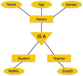
For example, the attributes of a Person class such as name, age, and gender can be inherited by lower-level entities such as Student or Teacher.

 

 

Key Differences between Generalization and Specialization in DBMS

1.      The fundamental difference between generalization and specialization is that Generalization is a bottom-up approach. However, specialization is a top-down approach.

2.      Generalization club all the entities that share some common properties to form a new entity. On the other hands, specialization spilt an entity to form multiple new entities that inherit some properties of the spiltted entity.

3.      In generalization, a higher entity must have some lower entities whereas, in specialization, a higher entity may not have any lower entity present.

4.      Generalization helps in reducing the size of schema whereas, specialization is just opposite it increases the number of entities thereby increasing the size of a schema.

5.      Generalization is always applied to the group of entities whereas, specialization is always applied on a single entity.

6.      Generalization results in a formation of a single entity whereas, Specialization results in the formation of multiple new entities.

ACID properties in DBMS

·         Atomicity - a transaction to transfer funds from one account to another involves making a withdrawal operation from the first account and a deposit operation on the second. If the deposit operation failed, you don’t want the withdrawal operation to happen either.

·         Consistency - a database tracking a checking account may only allow unique check numbers to exist for each transaction

·         Isolation - a teller looking up a balance must be isolated from a concurrent transaction involving a withdrawal from the same account. Only when the withdrawal transaction commits successfully and the teller looks at the balance again will the new balance be reported.

·         Durability - A system crash or any other failure must not be allowed to lose the results of a transaction or the contents of the database. Durability is often achieved through separate transaction logs that can "re-create" all transactions from some picked point in time (like a backup).

 

 

Update table

UPDATE table_name
SET column1 = value1, column2 = value2,
WHERE condition;

 

Example

UPDATE Customers
SET ContactName = 'Alfred Schmidt', City= 'Frankfurt'
WHERE CustomerID = 1;

 

How can delete column in sql

ALTER TABLE "table_name"
DROP COLUMN "column_name";

Table Customer

Column Name	Data Type
First_Name	char(50)
Last_Name	char(50)
Address	char(50)
City	char(50)
Country	char(25)
Birth_Date	datetime

Our goal is to drop the "Birth_Date" column. To do this, we key in:

MySQL: 

ALTER TABLE Customer DROP Birth_Date;

 

sql trigger example

 

Triggers are stored programs, which are automatically executed or fired when some events occur. Triggers are, in fact, written to be executed in response to any of the following events −

·         A database manipulation (DML) statement (DELETE, INSERT, or UPDATE)

·         A database definition (DDL) statement (CREATE, ALTER, or DROP).

·         A database operation (SERVERERROR, LOGON, LOGOFF, STARTUP, or SHUTDOWN).

Triggers can be defined on the table, view, schema, or database with which the event is associated.

Benefits of Triggers

Triggers can be written for the following purposes −

·         Generating some derived column values automatically

·         Enforcing referential integrity

·         Event logging and storing information on table access

·         Auditing

·         Synchronous replication of tables

·         Imposing security authorizations

·         Preventing invalid transactions

Creating Triggers

The syntax for creating a trigger is −

CREATE [OR REPLACE ] TRIGGER trigger_name  

{BEFORE | AFTER | INSTEAD OF }

{INSERT [OR]| UPDATE [OR]| DELETE}

[OF col_name]

ON table_name  

[REFERENCING OLD AS o NEW AS n]

[FOR EACH ROW]

WHEN (condition)

DECLARE 

Declaration-statements 

BEGIN

Executable-statements 

EXCEPTION 

Exception-handling-statements 

END;

Where,

·         CREATE [OR REPLACE] TRIGGER trigger_name − Creates or replaces an existing trigger with the trigger_name.

·         {BEFORE | AFTER | INSTEAD OF} − This specifies when the trigger will be executed. The INSTEAD OF clause is used for creating trigger on a view.

·         {INSERT [OR] | UPDATE [OR] | DELETE} − This specifies the DML operation.

·         [OF col_name] − This specifies the column name that will be updated.

·         [ON table_name] − This specifies the name of the table associated with the trigger.

·         [REFERENCING OLD AS o NEW AS n] − This allows you to refer new and old values for various DML statements, such as INSERT, UPDATE, and DELETE.

·         [FOR EACH ROW] − This specifies a row-level trigger, i.e., the trigger will be executed for each row being affected. Otherwise the trigger will execute just once when the SQL statement is executed, which is called a table level trigger.

·         WHEN (condition) − This provides a condition for rows for which the trigger would fire. This clause is valid only for row-level triggers.

Example

To start with, we will be using the CUSTOMERS table we had created and used in the previous chapters −

Select * from customers;  

+----+----------+-----+-----------+----------+ 

| ID | NAME     | AGE | ADDRESS   | SALARY   | 

+----+----------+-----+-----------+----------+ 

|  1 | Ramesh   |  32 | Ahmedabad |  2000.00 | 

|  2 | Khilan   |  25 | Delhi     |  1500.00 | 

|  3 | kaushik  |  23 | Kota      |  2000.00 | 

|  4 | Chaitali |  25 | Mumbai    |  6500.00 | 

|  5 | Hardik   |  27 | Bhopal    |  8500.00 | 

|  6 | Komal    |  22 | MP        |  4500.00 | 

+----+----------+-----+-----------+----------+ 

The following program creates a row-level trigger for the customers table that would fire for INSERT or UPDATE or DELETE operations performed on the CUSTOMERS table. This trigger will display the salary difference between the old values and new values −

CREATE OR REPLACE TRIGGER display_salary_changes 

BEFORE DELETE OR INSERT OR UPDATE ON customers 

FOR EACH ROW 

WHEN (NEW.ID >0)

DECLARE 

   sal_diff number;

BEGIN

   sal_diff :=:NEW.salary  -:OLD.salary;

   dbms_output.put_line('Old salary: '||:OLD.salary);

   dbms_output.put_line('New salary: '||:NEW.salary);

   dbms_output.put_line('Salary difference: '|| sal_diff);

END;

Advantages of using SQL triggers

·         SQL triggers provide an alternative way to check the integrity of data.

·         SQL triggers can catch errors in business logic in the database layer.

·         SQL triggers provide an alternative way to run scheduled tasks. By using SQL triggers, you don’t have to wait to run the scheduled tasks because the triggers are invoked automatically before or after a change is made to the data in the tables.

·         SQL triggers are very useful to audit the changes of data in tables.

Disadvantages of using SQL triggers

·         SQL triggers only can provide an extended validation and they cannot replace all the validations. Some simple validations have to be done in the application layer. For example, you can validate user’s inputs in the client side by using JavaScript or on the server side using server-side scripting languages such as JSP, PHP, ASP.NET, Perl.

·         SQL triggers are invoked and executed invisible from the client applications, therefore, it is difficult to figure out what happens in the database layer.

·         SQL triggers may increase the overhead of the database server.

how to get highest salary in each department

 

SQL Query to find department with highest number of employees

Get second highest salary

selectmax( salary ) from  emp

where salary not in ( select max ( salary ) from  emp );

 

Get third highest salary from employee table

 

Selectmax ( salary ) from  emp

Where salary not in (select max (salary) from emp

Where salary not in (select max (salary) from emp));

Given two tables are employee(id,name,salary, dept_id) and department(dept_id, dept_name),

Write a SQL to find MAX salary and AVERAGE Salary for Specific depnrtment [Dutch Bangla Bank -2017]

 

Select dept name, max(salary) from employee, department where employee.dept_id=department.dept_id  group by (dept_name);

 

Select dept_name,avg(salary) from employee,department where

employee.dept_id=department.dept_id group by (dept_name);

 

 

How to find Top Three Salaries from employee table ?

 

 

Or

SELECT Stuid, Stuname, AVG(Grade)AS GPA FROMTable

GROUPBY Stuid, Stuname

HAVING AVG(GRADE)>90

ORDERBY GPA DESC

 

Jibon binma question

 

Bcc ICT question:-

 

Students

Id	Name
1	Rahim
1	Rahim
2	Karim
2	Karim
3	Kamal
4	Jamal

Grade

Id	Sub_name	Marks
1	DBMS	56
1	Programming	72
2	AI	60
2	SE	70
3	AI	61
4	DBMS	85

 

 

Q1.SELECT Name,AVG(mark) FROM student JOIN grade ON student.id=grade.id GROUP BY Name DESC HAVING AVG(mark)<=64 

Name	AVG
karim	65
Jamal	85

 

Q2.SELECT Name,mark FROM student JOIN grade ON student.id=grade.id WHERE mark>=59

 

Given two tables are employee (id, name, salary, dept_id) and another table department (dept_id, dept_name), write SQL to find MAX salary and AVERAGE salary for specific department. [PO at Dutch bangla Bank]

 

select dept_id, MAX(salary ) as Max_salary, AVG(salary ) as avg_salary

from `empolyee`

group by dept_id;

 

 

Given two tables are employee (id, name, salary, dept_id) and another table department (dept_id, dept_name), write SQL to find MAX salary, AVERAGE salary and department name for each department. [PO at Dutch bangla Bank]

 

select e.dept_id, MAX(salary ) as Max_salary, AVG(salary ) as avg_salary, d.dept_name

 from `empolyee` e inner join `department` d on (e.dept_id=d.dept_id )

group by dept_id;

 

or

 

select e.dept_id, MAX(salary ) as Max_salary, AVG(salary ) as avg_salary, d.dept_name

 from `empolyee` e inner join `department` d on (e.dept_id=d.dept_id )

group by dept_name;

 

What is the SQL query for showing only the duplicate lists in student (stdid, name, gpa) table?

 

Select * from student

Where stdid in (select stdid

From student

Group by stdid

Having count(*)>1)

Top three salary

 

SELECT  *FROM

    (

 SELECT *FROM emp

    ORDER BY Salary desc

    )

WHERE rownum <= 3

ORDER BY Salary ;

 

Something like the following should do it.

 

SELECT  Name, Salary

FROM

    (

SELECT  Name, Salary

    FROM         emp

ORDER BY Salary desc

    )

WHERE rownum <= 3

ORDER BY Salary ;

 

Another Way :

 

select * from

    (

select empno,salary from emp

order by salary desc

    )

where rownum <= 3;

 

another way

 

SELECT  Name, Salary

FROM

    (

    SELECT  Name, Salary

FROM         emp

ORDER BY Salary desc

    )

WHERE rownum <= 3

ORDER BY Salary ;

 

 

Solution - 1

SELECT DISTINCT TOP 5 salary

FROM employee

ORDER BY salary DESC

 

 

Solution-2

 

select  * from employee where salary in (select distinct top 5 salary from employee order by salary desc)

 

solution -3

 

SELECT TOP 5 salary

FROM employee

ORDER BY salary DESC

 

Solution -10

SELECT *

FROM table

WHERE

(

  sal IN

  (

SELECT TOP (5) sal

FROM table as table1

GROUP BY sal

ORDER BY sal DESC

  )

)

 

 

DBMS - Hashing

 

For a huge database structure, it can be almost next to impossible to search all the index values through all its level and then reach the destination data block to retrieve the desired data. Hashing is an effective technique to calculate the direct location of a data record on the disk without using index structure.

Hashing uses hash functions with search keys as parameters to generate the address of a data record.

Hash Organization

·         Bucket − A hash file stores data in bucket format. Bucket is considered a unit of storage. A bucket typically stores one complete disk block, which in turn can store one or more records.

·         Hash Function − A hash function, h, is a mapping function that maps all the set of search-keys K to the address where actual records are placed. It is a function from search keys to bucket addresses.

Static Hashing

In static hashing, when a search-key value is provided, the hash function always computes the same address. For example, if mod-4 hash function is used, then it shall generate only 5 values. The output address shall always be same for that function. The number of buckets provided remains unchanged at all times.

Operation

·         Insertion − When a record is required to be entered using static hash, the hash function h computes the bucket address for search key K, where the record will be stored.

Bucket address = h(K)

·         Search − When a record needs to be retrieved, the same hash function can be used to retrieve the address of the bucket where the data is stored.

·         Delete − This is simply a search followed by a deletion operation.

Bucket Overflow

The condition of bucket-overflow is known as collision. This is a fatal state for any static hash function. In this case, overflow chaining can be used.

·         Overflow Chaining − When buckets are full, a new bucket is allocated for the same hash result and is linked after the previous one. This mechanism is called Closed Hashing.

·         Linear Probing − When a hash function generates an address at which data is already stored, the next free bucket is allocated to it. This mechanism is called Open Hashing.

Dynamic Hashing

The problem with static hashing is that it does not expand or shrink dynamically as the size of the database grows or shrinks. Dynamic hashing provides a mechanism in which data buckets are added and removed dynamically and on-demand. Dynamic hashing is also known as extended hashing.

Hash function, in dynamic hashing, is made to produce a large number of values and only a few are used initially.

Organization

The prefix of an entire hash value is taken as a hash index. Only a portion of the hash value is used for computing bucket addresses. Every hash index has a depth value to signify how many bits are used for computing a hash function. These bits can address 2n buckets. When all these bits are consumed − that is, when all the buckets are full − then the depth value is increased linearly and twice the buckets are allocated.

Operation

·         Querying − Look at the depth value of the hash index and use those bits to compute the bucket address.

·         Update − Perform a query as above and update the data.

·         Deletion − Perform a query to locate the desired data and delete the same.

·         Insertion − Compute the address of the bucket

o    If the bucket is already full.

§  Add more buckets.

§  Add additional bits to the hash value.

§  Re-compute the hash function.

o    Else

§  Add data to the bucket,

o    If all the buckets are full, perform the remedies of static hashing.

Hashing is not favorable when the data is organized in some ordering and the queries require a range of data. When data is discrete and random, hash performs the best.

Hashing algorithms have high complexity than indexing. All hash operations are done in constant time.

DBMS - Concurrency Control

In a multiprogramming environment where multiple transactions can be executed simultaneously, it is highly important to control the concurrency of transactions. We have concurrency control protocols to ensure atomicity, isolation, and serializability of concurrent transactions. Concurrency control protocols can be broadly divided into two categories −

·         Lock based protocols

·         Time stamp based protocols

Lock-based Protocols

Database systems equipped with lock-based protocols use a mechanism by which any transaction cannot read or write data until it acquires an appropriate lock on it. Locks are of two kinds −

·         Binary Locks − A lock on a data item can be in two states; it is either locked or unlocked.

·         Shared/exclusive − This type of locking mechanism differentiates the locks based on their uses. If a lock is acquired on a data item to perform a write operation, it is an exclusive lock. Allowing more than one transaction to write on the same data item would lead the database into an inconsistent state. Read locks are shared because no data value is being changed.

Timestamp-based Protocols

The most commonly used concurrency protocol is the timestamp based protocol. This protocol uses either system time or logical counter as a timestamp.

Lock-based protocols manage the order between the conflicting pairs among transactions at the time of execution, whereas timestamp-based protocols start working as soon as a transaction is created.

Thomas' Write Rule

This rule states if TS(Ti) < W-timestamp(X), then the operation is rejected and T_i is rolled back.

Time-stamp ordering rules can be modified to make the schedule view serializable.

Instead of making T_i rolled back, the 'write' operation itself is ignored.

 

Concurrency-control protocols : allow concurrent schedules, but ensure that the schedules are conflict/view serializable, and are recoverable and maybe even cascadeless.
These protocols do not examine the precedence graph as it is being created, instead a protocol imposes a discipline that avoids non-seralizable schedules.
Different concurrency control protocols provide different advantages between the amount of concurrency they allow and the amount of overhead that they impose.
We’ll be learning some protocols which are important for GATE CS. Questions from this topic is frequently asked and it’s recommended to learn this concept. (At the end of this series of articles I’ll try to list all theoretical aspects of this concept for students to revise quickly and they may find the material in one place.) Now, let’s get going:

Different categories of protocols:

§  Lock Based Protocol

·         Basic 2-PL

·         Conservative 2-PL

·         Strict 2-PL

·         Rigorous 2-PL

§  Graph Based Protocol

§  Time-Stamp Ordering Protocol

§  Multiple Granularity Protocol

§  Multi-version Protocol

Lock Based Protocols –
A lock is a variable associated with a data item that describes a status of data item with respect to possible operation that can be applied to it. They synchronize the access by concurrent transactions to the database items. It is required in this protocol that all the data items must be accessed in a mutually exclusive manner. Let me introduce you to two common locks which are used and some terminology followed in this protocol.

1.      Shared Lock (S): also known as Read-only lock. As the name suggests it can be shared between transactions because while holding this lock the transaction does not have the permission to update data on the data item. S-lock is requested using lock-S instruction.

2.      Exclusive Lock (X): Data item can be both read as well as written.This is Exclusive and cannot be held simultaneously on the same data item. X-lock is requested using lock-X instruction.

Lock Compatibility Matrix –

§  A transaction may be granted a lock on an item if the requested lock is compatible with locks already held on the item by other transactions.

§  Any number of transactions can hold shared locks on an item, but if any transaction holds an exclusive(X) on the item no other transaction may hold any lock on the item.

§  If a lock cannot be granted, the requesting transaction is made to wait till all incompatible locks held by other transactions have been released. Then the lock is granted.

§  Consider the Partial Schedule:

	T1	T2
1	lock-X(B)
2	read(B)
3	B:=B-50
4	write(B)
5		lock-S(A)
6		read(A)
7		lock-S(B)
8	lock-X(A)
9	……	……

§  Deadlock – consider the above execution phase. Now, T₁ holds an Exclusive lock over B, and T₂ holds a Shared lock over A. Consider Statement 7, T₁ requests for lock on B, while in Statement 8 T₂requests lock on A. This as you may notice imposes a Deadlock as none can proceed with their execution.

§  Starvation – is also possible if concurrency control manager is badly designed. For example: A transaction may be waiting for an X-lock on an item, while a sequence of other transactions request and are granted an S-lock on the same item. This may be avoided if the concurrency control manager is properly designed.

DBMS - Transaction

A transaction can be defined as a group of tasks. A single task is the minimum processing unit which cannot be divided further.

Let’s take an example of a simple transaction. Suppose a bank employee transfers Rs 500 from A's account to B's account. This very simple and small transaction involves several low-level tasks.

A’s Account	B’s Account
Open_Account(A) Old_Balance = A.balance New_Balance = Old_Balance - 500 A.balance = New_Balance Close_Account(A)	Open_Account(B) Old_Balance = B.balance New_Balance = Old_Balance + 500 B.balance = New_Balance Close_Account(B)

States of Transactions

A transaction in a database can be in one of the following states −

·         Active − In this state, the transaction is being executed. This is the initial state of every transaction.

·         Partially Committed − When a transaction executes its final operation, it is said to be in a partially committed state.

·         Failed − A transaction is said to be in a failed state if any of the checks made by the database recovery system fails. A failed transaction can no longer proceed further.

·         Aborted − If any of the checks fails and the transaction has reached a failed state, then the recovery manager rolls back all its write operations on the database to bring the database back to its original state where it was prior to the execution of the transaction. Transactions in this state are called aborted. The database recovery module can select one of the two operations after a transaction aborts −

o    Re-start the transaction

o    Kill the transaction

·         Committed − If a transaction executes all its operations successfully, it is said to be committed. All its effects are now permanently established on the database system.

ERD(constraint) Entity relationship diagram

What is an Entity Relationship Diagram (ERD)?

An entity relationship diagram (ERD) shows the relationships of entity sets stored in a database. An entity in this context is a component of data. In other words, ER diagrams illustrate the logical structure of databases.

At first glance an entity relationship diagram looks very much like a flowchart. It is the specialized symbols, and the meanings of those symbols, that make it unique.

Use also ConceptDraw DIAGRAM v12 enhanced with powerful Entity-Relationship Diagram (ERD) solution to draw your own ER diagrams using Chen's notation icons.

Symbol		Shape Name		Symbol Description
Entities
		Entity		An entity is represented by a rectangle which contains the entity’s name.
		Weak Entity		An entity that cannot be uniquely identified by its attributes alone. The existence of a weak entity is dependent upon another entity called the owner entity. The weak entity’s identifier is a combination of the identifier of the owner entity and the partial key of the weak entity.
		Associative Entity		An entity used in a many-to-many relationship (represents an extra table). All relationships for the associative entity should be many
Attributes
		Attribute	In the Chen notation, each attribute is represented by an oval containing atributte’s name
		Key attribute	An attribute that uniquely identifies a particular entity. The name of a key attribute is underscored.
		Multivalued attribute	An attribute that can have many values (there are many distinct values entered for it in the same column of the table). Multivalued attribute is depicted by a dual oval.
		Derived attribute	An attribute whose value is calculated (derived) from other attributes. The derived attribute may or may not be physically stored in the database. In the Chen notation, this attribute is represented by dashed oval.
Relationships
	Strong relationship		A relationship where entity is existence-independent of other entities, and PK of Child doesn’t contain PK component of Parent Entity. A strong relationship is represented by a single rhombus
	Weak (identifying) relationship		A relationship where Child entity is existence-dependent on parent, and PK of Child Entity contains PK component of Parent Entity. This relationship is represented by a double rhombus.

 

Types of Attributes in dbms

·         Single valued attributes

·         Multi valued attributes

·         Compound /Composite attributes

·         Simple / Atomic attributes

·         Stored attributes

·         Derived attributes

·         Complex attributes

·         Key attributes

·         Non key attributes

·         Required attributes

·         Optional/ null value attribute

Strong Entity Set	Weak Entity Set
Strong entity set always has a primary key.	It does not have enough attributes to build a primary key.
It is represented by a rectangle symbol.	It is represented by a double rectangle symbol.
It contains a Primary key represented by the underline symbol.	It contains a Partial Key which is represented by a dashed underline symbol.
The member of a strong entity set is called as dominant entity set.	The member of a weak entity set called as a subordinate entity set.
Primary Key is one of its attributes which helps to identify its member.	In a weak entity set, it is a combination of primary key and partial key of the strong entity set.
In the ER diagram the relationship between two strong entity set shown by using a diamond symbol.	The relationship between one strong and a weak entity set shown by using the double diamond symbol.
The connecting line of the strong entity set with the relationship is single.	The line connecting the weak entity set for identifying relationship is double.

difference between indexing and hashing?

Hash is sort of an index: it can be used to locate a record based on a key -- but it doesn't preserve any order of records. Based on hash, one can't iterate to the succeeding or preceding element. This is however, what index does (in the context of databases.)

Q. What is indexing in database? Differentiate between cluster and non-cluster indexing.[eastern refinery -2016]

Indexing in Databases | Set 1

Indexing is a way to optimize performance of a database by minimizing the number of disk accesses required when a query is processed.

An index or database index is a data structure which is used to quickly locate and access the data in a database table.

Indexes are created using some database columns.

§  The first column is the Search key that contains a copy of the primary key or candidate key of the table. These values are stored in sorted order so that the corresponding data can be accessed quickly (Note that the data may or may not be stored in sorted order).

§  The second column is the Data Reference which contains a set of pointers holding the address of the disk block where that particular key value can be found.

There are two kinds of indices:

1.      Ordered indices: Indices are based on a sorted ordering of the values.

2.      Hash indices: Indices are based on the values being distributed uniformly across a range of buckets. The buckets to which a value is assigned is determined by function called a hash function.

There is no comparison between both the techniques, it depends on the database application on which it is being applied.

§  Access Types: e.g. value based search, range access, etc.

§  Access Time: Time to find particular data element or set of elements.

§  Insertion Time: Time taken to find the appropriate space and insert a new data time.

§  Deletion Time: Time taken to find an item and delete it as well as update the index structure.

§  Space Overhead: Additional space required by the index.

Indexing Methods

Ordered Indices

The indices are usually sorted so that the searching is faster. The indices which are sorted are known as ordered indices.

§  If the search key of any index specifies same order as the sequential order of the file, it is known as primary index or clustering index.
Note: The search key of a primary index is usually the primary key, but it is not necessarily so.

§  If the search key of any index specifies an order different from the sequential order of the file, it is called the secondary index or non-clustering index.

Clustered Indexing

Clustering index is defined on an ordered data file. The data file is ordered on a non-key field. In some cases, the index is created on non-primary key columns which may not be unique for each record. In such cases, in order to identify the records faster, we will group two or more columns together to get the unique values and create index out of them. This method is known as clustering index. Basically, records with similar characteristics are grouped together and indexes are created for these groups.

For example, students studying in each semester are grouped together. i.e. 1^st Semester students, 2^nd semester students, 3^rdsemester students etc are grouped.

​Clustered index sorted according to first name (Search key)

Primary Index​​

In this case, the data is sorted according to the search key. It induces sequential file organisation.
In this case, the primary key of the database table is used to create the index. As primary keys are unique and are stored in sorted manner, the performance of searching operation is quite efficient. The primary index is classified into two types : Dense Index and Sparse Index.

(I) Dense Index : ​

§  For every search key value in the data file, there is an index record.

§  This record contains the search key and also a reference to the first data record with that search key value.

(II) Sparse Index :

§ 
The index record appears only for a few items in the data file. Each item points to a block as shown.

§  To locate a record, we find the index record with the largest search key value less than or equal to the search key value we are looking for.

§  We start at that record pointed to by the index record, and proceed along the pointers in the file (that is, sequentially) until we find the desired record.

 

Non­-Clustered Indexing

​A non clustered index just tells us where the data lies, i.e. it gives us a list of virtual pointers or references to the location where the data is actually stored. Data is not physically stored in the order of the index. Instead , data is present in leaf nodes. For eg. the contents page of a book. Each entry gives us the page number or location of the information stored. The actual data here(information on each page of book) is not organised but we have an ordered reference(contents page) to where the data points actually lie.

It requires more time as compared to clustered index because some amount of extra work is done in order to extract the data by further following the pointer. In case of clustered index, data is directly present in front of the index.

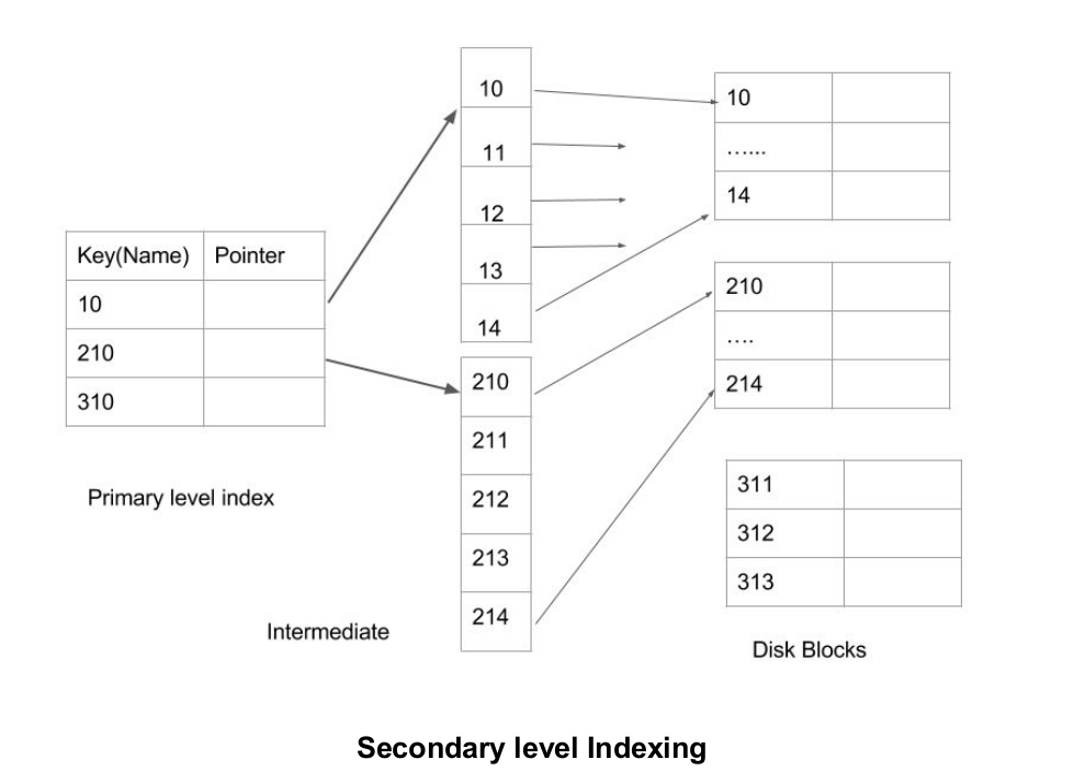
Secondary Index​

It is used to optimize query processing and access records in a database with some information other than the usual search key (primary key). In this two levels of indexing are used in order to reduce the mapping size of the first level and in general. Initially, for the first level, a large range of numbers is selected so that the mapping size is small. Further, each range is divided into further sub ranges.

In order for quick memory access, first level is stored in the primary memory. Actual physical location of the data is determined by the second mapping level.

 

Another part of description :

·         Primary Index − Primary index is defined on an ordered data file. The data file is ordered on a key field. The key field is generally the primary key of the relation.

·         Secondary Index − Secondary index may be generated from a field which is a candidate key and has a unique value in every record, or a non-key with duplicate values.

·         Clustering Index − Clustering index is defined on an ordered data file. The data file is ordered on a non-key field.

Ordered Indexing is of two types −

·         Dense Index

·         Sparse Index

Dense Index

In dense index, there is an index record for every search key value in the database. This makes searching faster but requires more space to store index records itself. Index records contain search key value and a pointer to the actual record on the disk.

Sparse Index

In sparse index, index records are not created for every search key. An index record here contains a search key and an actual pointer to the data on the disk. To search a record, we first proceed by index record and reach at the actual location of the data. If the data we are looking for is not where we directly reach by following the index, then the system starts sequential search until the desired data is found.

Multilevel Index

Index records comprise search-key values and data pointers. Multilevel index is stored on the disk along with the actual database files. As the size of the database grows, so does the size of the indices. There is an immense need to keep the index records in the main memory so as to speed up the search operations. If single-level index is used, then a large size index cannot be kept in memory which leads to multiple disk accesses.

Multi-level Index helps in breaking down the index into several smaller indices in order to make the outermost level so small that it can be saved in a single disk block, which can easily be accommodated anywhere in the main memory.

what is the technical difference between 32 bit and 64 bit operating system? [BUET madrasha board-2018]

The terms 32-bit and 64-bit refer to the way a computer's processor (also called a CPU), handles information. The 64-bit version of Windows handles large amounts of random access memory (RAM) more effectively than a 32-bit system. 

Difference between 32-bit and 64-bit operating systems

In computing, there exist two type processor i.e., 32-bit and 64-bit. These processor tells us how much memory a processor can have access from a CPU register. For instance,

A 32-bit system can access 2³² memory addresses, i.e 4 GB of RAM or physical memory.
A 64-bit system can access 2⁶⁴ memory addresses, i.e actually 18-Billion GB of RAM. In short, any amount of memory greater than 4 GB can be easily handled by it.

 

Difference between clustered and nonclustered indexing? [eastern refinery buet-2016]

Clustered Index

·         Only one per table

·         Faster to read than non clustered as data is physically stored in index order

Non Clustered Index

·         Can be used many times per table

·         Quicker for insert and update operations than a clustered index

Both types of index will improve performance when select data with fields that use the index but will slow down update and insert operations.

Because of the slower insert and update clustered indexes should be set on a field that is normally incremental ie Id or Timestamp.

SQL Server will normally only use an index if its selectivity is above 95%.

Microsoft Answer: -

A table or view can contain the following types of indexes:

1.       Clustered

Ø  Clustered indexes sort and store the data rows in the table or view based on their key values. These are the columns included in the index definition. There can be only one clustered index per table, because the data rows themselves can be stored in only one order.

Ø  The only time the data rows in a table are stored in sorted order is when the table contains a clustered index. When a table has a clustered index, the table is called a clustered table. If a table has no clustered index, its data rows are stored in an unordered structure called a heap.

2.       Nonclustered

Ø  Nonclustered indexes have a structure separate from the data rows. A nonclustered index contains the nonclustered index key values and each key value entry has a pointer to the data row that contains the key value.

Ø  The pointer from an index row in a nonclustered index to a data row is called a row locator. The structure of the row locator depends on whether the data pages are stored in a heap or a clustered table. For a heap, a row locator is a pointer to the row. For a clustered table, the row locator is the clustered index key.

difference between cluster and non cluster index in database

Clustered Index

·         Only one per table

·         Faster to read than non clustered as data is physically stored in index order

Non Clustered Index

·         Can be used many times per table

·         Quicker for insert and update operations than a clustered index

Both types of index will improve performance when select data with fields that use the index but will slow down update and insert operations.

Because of the slower insert and update clustered indexes should be set on a field that is normally incremental ie Id or Timestamp.

SQL Server will normally only use an index if its selectivity is above 95%.

Clustered Index

A clustered index defines the order in which data is physically stored in a table. Table data can be sorted in only way, therefore, there can be only one clustered index per table. In SQL Server, the primary key constraint automatically creates a clustered index on that particular column.

Let’s take a look. First, create a “student” table inside “schooldb” by executing the following script:

CREATE DATABASE schooldb                                                   

CREATE TABLE student

(

    id INT PRIMARY KEY,

    name VARCHAR(50) NOT NULL,

    gender VARCHAR(50) NOT NULL,

    DOB datetime NOT NULL,

    total_score INT NOT NULL,

    city VARCHAR(50) NOT NULL

 )

Notice here in the “student” table we have set primary key constraint on the “id” column. This automatically creates a clustered index on the “id” column. To see all the indexes on a particular table execute “sp_helpindex” stored procedure. This stored procedure accepts the name of the table as a parameter and retrieves all the indexes of the table. The following query retrieves the indexes created on student table.

USE schooldb                                                         

EXECUTE sp_helpindex student

The above query will return this result:

index_name                                 index_description                                                            index_keys

PK__student__3213E83F7F60ED59   clustered, unique, primary key located on PRIMARY     id

Non-Clustered Indexes

A non-clustered index doesn’t sort the physical data inside the table. In fact, a non-clustered index is stored at one place and table data is stored in another place. This is similar to a textbook where the book content is located in one place and the index is located in another. This allows for more than one non-clustered index per table.

When a query is issued against a column on which the index is created, the database will first go to the index and look for the address of the corresponding row in the table. It will then go to that row address and fetch other column values. It is due to this additional step that non-clustered indexes are slower than clustered indexes.

Creating a Non-Clustered Index

The syntax for creating a non-clustered index is similar to that of clustered index. However, in case of non-clustered index keyword “NONCLUSTERED” is used instead of “CLUSTERED”. Take a look at the following script.

use schooldb

CREATE NONCLUSTERED INDEX IX_tblStudent_Name

ON student(name ASC)

The above script creates a non-clustered index on the “name” column of the student table. The index sorts by name in ascending order. As we said earlier, the table data and index will be stored in different places. The table records will be sorted by a clustered index if there is one. The index will be sorted according to its definition and will be stored separately from the table.

Student Table Data:

id      name    gender             DOB                                       total_score                   City

1        Jolly     Female 1989-06-12 00:00:00.000                    500                              London

2        Jon       Male                1974-02-02 00:00:00.000        545                              Manchester

3        Sara     Female 1988-03-07 00:00:00.000                    600                              Leeds

4        Laura   Female 1981-12-22 00:00:00.000                    400                              Liverpool

5        Alan    Male                1993-07-29 00:00:00.000        500                              London

6        Kate    Female 1985-01-03 00:00:00.000                       500                              Liverpool

IX_tblStudent_Name Index Data

name             Row Address

Alan              Row Address

Elis                Row Address

Jolly              Row Address

Jon                Row Address

Joseph           Row Address

Kate              Row Address

 here in the index every row has a column that stores the address of the row to which the name belongs. So if a query is issued to retrieve the gender and DOB of the student named “Jon”, the database will first search the name “Jon” inside the index.

 

Why indexing is used in database?How hash table works?       [DESCO BUET Asst. Eng 2016]

 

An index is just a data structure that makes the searching faster for a specific column in a database. This structure is usually a b-tree or a hash table but it can be any other logic structure.

How a database index can help performance

The whole point of having an index is to speed up search queries by essentially cutting down the number of records/rows in a table that need to be examined. An index is a data structure (most commonly a B- tree) that stores the values for a specific column in a table.

How does B-trees index work?

The reason B- trees are the most popular data structure for indexes is due to the fact that they are time efficient – because look-ups, deletions, and insertions can all be done in logarithmic time. And, another major reason B- trees are more commonly used is because the data that is stored inside the B- tree can be sorted. The RDBMS typically determines which data structure is actually used for an index. But, in some scenarios with certain RDBMS’s, you can actually specify which data structure you want your database to use when you create the index itself.

Q1. (i) Which type of JOIN is used to find not matched data from table?

Here's a simple query:

SELECT t1.ID

FROM Table1 t1

LEFTJOIN Table2 t2 ON t1.ID = t2.ID

WHERE t2.ID ISNULL

The key points are:

1.      LEFT JOIN is used; this will return ALL rows from Table1, regardless of whether or not there is a matching row in Table2.

2.      The WHERE t2.ID IS NULL clause; this will restrict the results returned to only those rows where the ID returned from Table2 is null - in other words there is NO record in Table2 for that particular ID from Table1. Table2.IDwill be returned as NULL for all records from Table1where the ID is not matched in Table2.

 (ii) In which keyword is used for retrieving data from table without duplicate row data?

I have a table with 3 columns like this:

+------------+---------------+-------+  

| Country_id | country_title | State |

+------------+---------------+-------+    

There are many records in this table. Some of them have state and some other don't. Now, imagine these records:

1| Canada  | Alberta  

2|  Canada | British  Columbia  

3| Canada  | Manitoba  

4| China   |

I need to have country names without any duplicate. Actually I need their id and title, What is the best SQL command to make this? I used DISTINCT in the form below but I could not achieve an appropriate result.

SELECTDISTINCT title,id FROM tbl_countries ORDERBY title

My desired result is something like this:

1, Canada  

4, China

 (iii) What is the output of the following query –   

        SELECT  *

         FROM myTbale

        WHERE id>0

        ORDER BY id DESC, NAME DESC

 

 

Flights(flno: integer, from: string, to: string, distance: integer, departs: time, arrives:time, price: real)
Aircraft(aid: integer, aname: string, cruisingrange: integer)
Certified(eid:integer, aid: integer)
Employees( eid: integer, ename: string, salary: integer)
For the schema above, write SQL to implement the following queries:
(i) Find the names of aircraft such that all pilots certified to operate them have salaries more than $80,000.
(ii) For each pilot who is certified for more than three aircraft, find the eid and the maximum cruisingrange of the aircraft for which she or he is certified.
(iii) Find the names of pilots whose salary is less than the price of the cheapest route from 'Los Angeles' to 'Honolulu'.
(iv) Find the aids of all aircraft that can be used on routes from 'Los Angeles' to 'Chicago'.
(v) Identify the routes that can be piloted by every pilot who makes more than $100,000.

Ans i) select distinct a.aname from aircraft a join certified c on a.aid=c.aid where c.eid IN (select e.eid from employees e join certified c on e.eid=c.eid where  `salary`>80000);

Or) select distinct a.aname from aircraft a join certified c on a.aid=c.aid join employees e on c.eid = e.eid where  `salary`>80000;

Or) SELECT DISTINCT a.aname FROM aircraft a,certified c,employees e WHERE a.aid=c.aid AND c.eid=e.eid AND NOT EXISTS (SELECT * FROM employees e1 WHERE e1.eid=e.eid AND e1.salary<80000);

ii) select c.eid, max(a.cruisingrange) from aircraft a join certified c on a.aid = c.aid group by c.eid having 3<count(c.eid);

or) SELECT c.eid,MAX(cruisingrange) FROM certified c,aircraft a WHERE c.aid=a.aid GROUP BY c.eid HAVING COUNT(*)>3;

iii) select distinct ename from employees where salary < (select min(price) from flight where `from` = 'Los Angeles' and `to` = 'Honolulu');

iv) SELECT aid FROM Aircraft WHERE cruisingrange > ( SELECT MIN (distance) FROM Flights WHERE `from` = 'Los Angeles' AND `to` = 'Chicago' );

Suppliers(sid: integer, sname: string, address: string)
Parts(pid: integer, pname: string, color: string)
Catalog(sid: integer, pid: integer, cost: real)
For the schema above, write down the Relational Algebric expression for the following
(i) Find the sids of suppliers who supply some red or green part.
(ii) Find the sids of suppliers who supply some red parts are atthe address 221 Packer
Street.
(iii) Find the sids of suppliers who supply some red parts and some green parts.
(iv) Find the sids of suppliers who supply every part.

Ans i) SELECT DISTINCT C.sid FROM Catalog C, Parts P WHERE C.pid = P.pid AND P.color = ‘Red’ UNION SELECT DISTINCT C1.sid FROM Catalog C1, Parts P1 WHERE C1.pid = P1.pid AND P1.color = ‘Green’

ii) SELECT distinct S.sid FROM Supliers S WHERE S.address =’221 Packer Street’ and S.sid IN( SELECT DISTINCT C.sid FROM Catalog C, Parts P WHERE C.pid = P.pid AND P.color = ‘Red’)

IIi) SELECT DISTINCT C.sid FROM Catalog C, Parts P WHERE C.pid = P.pid AND P.color = ‘Red’ INTERSECT SELECT DISTINCT C1.sid FROM Catalog C1, Parts P1 WHERE C1.pid = P1.pid AND P1.color = ‘Green’

iv) SELECT S.sid FROM Supliers S WHERE NOT EXISTS ((SELECT P.pid FROM Parts P) EXCEPT (SELECT C.pid FROM Catalog C WHERE C.sid=S.sid))

Which two ACID properties are maintained by the Recovery Manager of a DBMS? C
Ans: The Recovery Manager is responsible for ensuring Atomicity and Durability

Atomicity is guaranteed by undoing the actions of the transactions that did not commit (aborted).

Durability is guaranteed by making sure that all actions of committed transactions survive crashes and failures.

) Consider the following relational schema:
employee (emp no, name, office, age)
books (isbn, title, author, publisher)
loan (empno, isbn, date)
where the primary keys are underlined.
Answer the following queries in relational algebra:
(i) Find the names of employees who have borrowed a book published by McGraw-Hill.
(ii) Find the names and ages of employees who have borrowed all books written by Carl Hamacher.
(iii) Find the names of employees who have borrowed more than five different books published by Pearson Education.
(iv) For each publisher, find the names of employees who have borrowed more than five books of that publisher.
(v) Find the titles and authors of the books that have been borrowed by Peter Hart.

Ans i) select name from employee e, books b, loan l where e.empno = l.empno and l.isbn = b.isbn and b.publisher = 'McGrawHill'

ii) select name from employee e join loan l on e.empno=l.empno join (select isbn from books where author = 'Carl Hamacher') x on l.isbn=x.isbn group by e.empno,name having count(*)= (select count(*) from books where author = 'Carl Hamacher')

iii) select name from employee,loan where employee.empno=loan.empno and isbn in ( select distinct isbn from books where publisher='McGraw-Hill') group by employee.empno,name having count(isbn) >=5

iv)select name from employee,loan,books where employee.empno=loan.empno and books.isbn=loan.isbn  group by employee.empno, name,books.publisher having count(loan.isbn) >=5

EMPLOYEE (EMPLOYEED, LASTNAME. FIRSTNAME, PHONE, HIREDATE,
JOBJD, SALARY, DEPARTMENT)
JOB (JOBID, JOBTITLE, MINSALARY, MAXSALARY)
DEPARTMENT (DEPARTMENTID, DEPARTMENTNAME, MANAGERID)
For the schema above, "write down the Relational algebra  expression for the following:
(i) List the average salary of each department.
(ii) List the FIRSTNAME and JOBTITLE of employee 'John',
(iii) Increase all salary more than 1000  by 5% and less than 10000 by 4%.
(iv) Delete all employees  from EMPLOYEE table who earn less than 1000 as salary.

Ans i) SELECT E.DEPARTMENT, AVG(E.SALARY) FROM EMPLOYEE E JOIN DEPARTMENT D ON E.DEPARTMENT = D.DEPARTMENTNAME GROUP BY E.DEPARTMENT

iv) Delete FROM Employee WHERE SALARY<1000

 

Source:

Tutorial point- https://www.tutorialspoint.com/

Java T point- https://www.javatpoint.com/

Geeksforgeeks- https://www.geeksforgeeks.org

 Techopedia - https://www.techopedia.com/

guru99- https://www.guru99.com/

techterms - https://techterms.com/

webopedia - https://www.webopedia.com/

study - https://study.com/

wikipedia - https://en.wikipedia.org/

cprogramming - https://www.cprogramming.com/

w3schools - https://www.w3schools.com/

Electronic hub- https://www.electronicshub.org/